ORA enrichment - single cell metabolomics • S2IsoMEr

Single-cell metabolomics generates output similar to scRNA-Seq, resulting in a matrix of metabolites (m) by cells (c), where values represent the abundance of each metabolite per cell. As with any single-cell analysis pipeline, enrichment analysis is typically one of the final steps to interpret the differential markers identified earlier.

Overrepresentation analysis (ORA) is the most common enrichment method for both bulk and single-cell datasets, regardless of the molecular readout. In metabolomics, several methods exist for metabolite enrichment, with MetaboAnalyst being the most popular. MetaboAnalyst is a robust platform offering various analyses for metabolomics data at different stages (raw, preprocessed, biomarkers, etc.). We recommend users explore this tool for additional analyses beyond enrichment.

For MS1-based metabolomics datasets, particularly in imaging MS, the inherent molecular ambiguity in metabolite identification complicates downstream analyses, including enrichment. To our knowledge, no other metabolite enrichment method addresses isomeric/isobaric ambiguity in enrichment analyses.

In this notebook, we demonstrate how to use S2IsoMEr for ORA enrichment in single-cell metabolomics datasets while accounting for isomeric/isobaric ambiguity.

Loading packages

library(S2IsoMEr)
library(dplyr)
library(tidyr)
library(ggplot2)

Dataset

The single-cell dataset used is from the SpaceM paper, which models NASH by stimulating Hepa-RG cells with fatty acids and other inhibitors compared to a control, followed by MALDI imaging MS.

The data is freely available in MetaboLights.

Download single-cell matrices and associated metadata

NASH_scm contains the single-cell metabolite matrix which will be main input as well as condition per cell in NASH_scm$metadata. These are the main required files to run single-cell metabolomics enrichment. condition_metadata contains the METASPACE dataset names for each replicate, while metaspace_annotations contains the annotation results for each dataset in the SpaceM project on METASPACE. We will use the annotation results and corresponding FDR thresholds to select metabolites as input query and corresponding universe for enrichment.

NASH_scm_tmp = tempfile()
download.file("https://zenodo.org/records/13318721/files/NASH_scm_dataset.rds", destfile = NASH_scm_tmp)
NASH_scm = readRDS(NASH_scm_tmp)

condition_metadata_tmp = tempfile()
download.file("https://zenodo.org/records/13318721/files/spacem_scm_matrices.rds", destfile = condition_metadata_tmp)
condition_metadata = readRDS(condition_metadata_tmp)[["metaspace_dataset_names"]]

metaspace_annotations_tmp = tempfile()
download.file("https://zenodo.org/records/13318721/files/SpaceM_metaspace_ds_annotations.rds", destfile = metaspace_annotations_tmp)
metaspace_annotations = readRDS(metaspace_annotations)

Prepare the input data

scm = NASH_scm$scm %>% 
  as.matrix() %>% 
  t()
conds = NASH_scm$metadata %>%
  column_to_rownames("Cell")
conds = conds[colnames(scm),]

conds_unique = conds %>% 
  dplyr::distinct()

metaspace_annotations = metaspace_annotations %>% 
  dplyr::left_join(condition_metadata, by = c("ds_name" = "dataset_name")) %>%
  dplyr::rename("Replicate" = "Condition") %>%
  dplyr::left_join(conds_unique)

Filter metabolites and specify conditions

Here we specify the reference and query conditions as cond_x and cond_y, respectively. And since METASPACE provides FDR-controlled annotations, we will select annotations passing desired_fdr as query and all detected annotations for a given annotation database (desired_annot_db) as custom universe.

cond_x = "U"
cond_y = "F"
desired_fdr = 0.1
desired_annot_db = "HMDB"

annots_des_fdr = metaspace_annotations %>%
  dplyr::filter(Condition %in% c(cond_x, cond_y),
                fdr <= desired_fdr,
                str_detect(db, desired_annot_db)) %>%
  pull(formula_adduct) %>%
  intersect(rownames(scm))

custom_univ = metaspace_annotations %>%
  dplyr::filter(Condition %in% c(cond_x, cond_y),
                str_detect(db, desired_annot_db)) %>%
  pull(formula_adduct) %>%
  intersect(rownames(scm))

input_scm = scm[annots_des_fdr,]

Initialize enrichment object

The first step is creating a S2IsoMEr object which contains the input matrix in scmatrix and the conditions for each cell specified in conditions. We need to specify the enrichment_type as “ORA”. annot_db corresponds to the annotation database used during the annotation, more relevant if annotation is performed using METASPACE. The databases supported are (“CoreMetabolome”, “HMDB”,“SwissLipids”,“LipidMaps”), if you want to provide a custom annotation database, you can provide it using annot_custom_db argument. Here we will use “HMDB” as annotation database.

Since we want to consider isomeric/isobaric ambiguity, we set either consider_isomers or consider_isobars to TRUE. If both were set to FALSE, it will run classic ORA with no bootstrapping. We also specify polarization_mode to positive since these datasets were acquired in positive mode.

For enrichment background, we use the background_type argument to select one of the possible background types :

LION : Uses LION ontology. Only for Lipids.
The following types are curated from RAMP-DB 2.0 :
1. super_class : Most coarse-grained classification
2. main_class : Fine-grained sub classification compared to super_class
3. sub_class : Most fine_grained sub classification.
4. pathways : Biological pathways curated from KEGG, HMDB, Reactome and WikiPathways.

We also specify the background molecule_type by specifying either Metabo for metabolites or Lipid for lipids. To pull the relevant background which is internally built in initEnrichment, you can provide the previous arguments to the Load_background function to get list of terms and their associated molecules as follows :

bg = Load_background(mol_type = "Metabo",
                     bg_type = "sub_class", 
                     feature_type = "name")

Finally we specify condition.x and condition.y as reference and query conditions, respectively. While running ORA in Run_enrichment, fold changes will be computed in condition.y relative to condition.x.

ORA_boot_obj = initEnrichment(scmatrix = input_scm, conditions = conds$Condition,
                     enrichment_type = "ORA",annot_db = "HMDB",
                     consider_isomers = T, consider_isobars = T,
                     polarization_mode = "positive",
                     background_type = "sub_class",
                     molecule_type = "Metabo",
                     condition.x = cond_x,
                     condition.y = cond_y)

There are additional arguments to initEnrichment that could be used depending on your dataset metadata and any other prior knowledge. Check documentation of ?initEnrichment for more information on these arguments.

Running ORA bootstrapping-based enrichment

Based on the initialized object, we provide Run_enrichment function as a wrapper around the main enrichment functions :

So you can also provide additional arguments to Run_enrichment from the argument list of the relevant function from the above list.

In this example, Run_enrichment will first calculate log fold change to separate metabolites into upregulated and downregulated if Run_DE is set to FALSE. If it was set to TRUE, the function seurat_WilcoxDETest (a wrapper for WilcoxDETest from Seurat) will be used to calculate p-values based on a wilcoxon rank-sum test which will be used in addition to the previously computed log fold changes to select the markers for ORA based on the DE_pval_cutoff and DE_LFC_cutoff arguments in the Run_enrichment function.

The min.pct.diff argument of 0.1 specifies that a marker must have at least a 10% difference in detection between cells in both conditions to be considered differentially abundant.

From the additional list of arguments to Run_bootstrap_ORA we recommend defining the following arguments to Run_enrichment :

custom_universe : List of background metabolites to be used. More specifically, these represent the set of all possible metabolites that were measured in a given dataset (optionally under a given threshold). If not provided, all metabolites in the selected background will be used and it might lead to potentially misleading results.
report_ambiguity_scores : Useful to understand the degree of isomeric/isobaric ambiguity per metabolite.
n_bootstraps: Number of bootstrap iterations. The default is 50, but increasing this number generally improves accuracy, though it will slow down the process. Adjust according to your needs. We recommend a minimum of 50 and a maximum of 1000. 100 is acceptable.

ORA_boot_res = Run_enrichment(object = ORA_obj,
                         custom_universe = custom_univ,
                         report_ambiguity_scores = T,
                         DE_LFC_cutoff = 0,min.pct.diff = 0)

Output

The main output of Run_bootstrap_ORA is a list of 2 dataframes :

“unfiltered_enrich_res” (ORA_boot_res[["unfiltered_enrich_res"]]) : Data frame containing the enrichment results for each term and bootstrap and the contingency table used for ORA.
“clean_enrich_res” (ORA_boot_res[["clean_enrich_res"]]): Summary statistics per term passing the filters specified in Run_bootstrap_ORA

Check ?Run_bootstrap_ORA for more information on the output and other parameters.

Since we used Run_enrichment as a wrapper around Run_bootstrap_ORA we get the ORA results separately for upregulated, downregulated, and all metabolites based on the calculated DE_LFC_cutoff specified above. If you use Run_bootstrap_ORA directly, you can provide a list of multiple conditions as input directly as long as you know the markers a priori.

To get a summary of the terms passing each filter, we can call passed_filters_per_term function on any unfiltered dataframe and any combinations of filters to understand why a given term was excluded in the final summarized results. Check ?passed_filters_per_term for more information on the filters.

enrich_ORA_summary = passed_filters_per_term(unfiltered_df = ORA_boot_res$upregulated$unfiltered_enrich_res,
                        enrich_type = "ORA", min_intersection = 3,alpha_cutoff = 0.05,q.val_cutoff = 0.2,boot_fract_cutoff = 0.5)
enrich_ORA_summary = enrich_ORA_summary[order(enrich_ORA_summary$pass_all_filts, decreasing = T),]
head(enrich_ORA_summary)

Visualization

Barplot

barplot_ORA_boot(ORA_boot_res = ORA_boot_res,collapse_multi_cond = T)

Dotplot

multi_cond_collapse = collapse_ORA_boot_multi_cond(ORA_boot_res_list = ORA_boot_res)
dotplot_ORA(ORA_res = multi_cond_collapse$clean_enrich_res)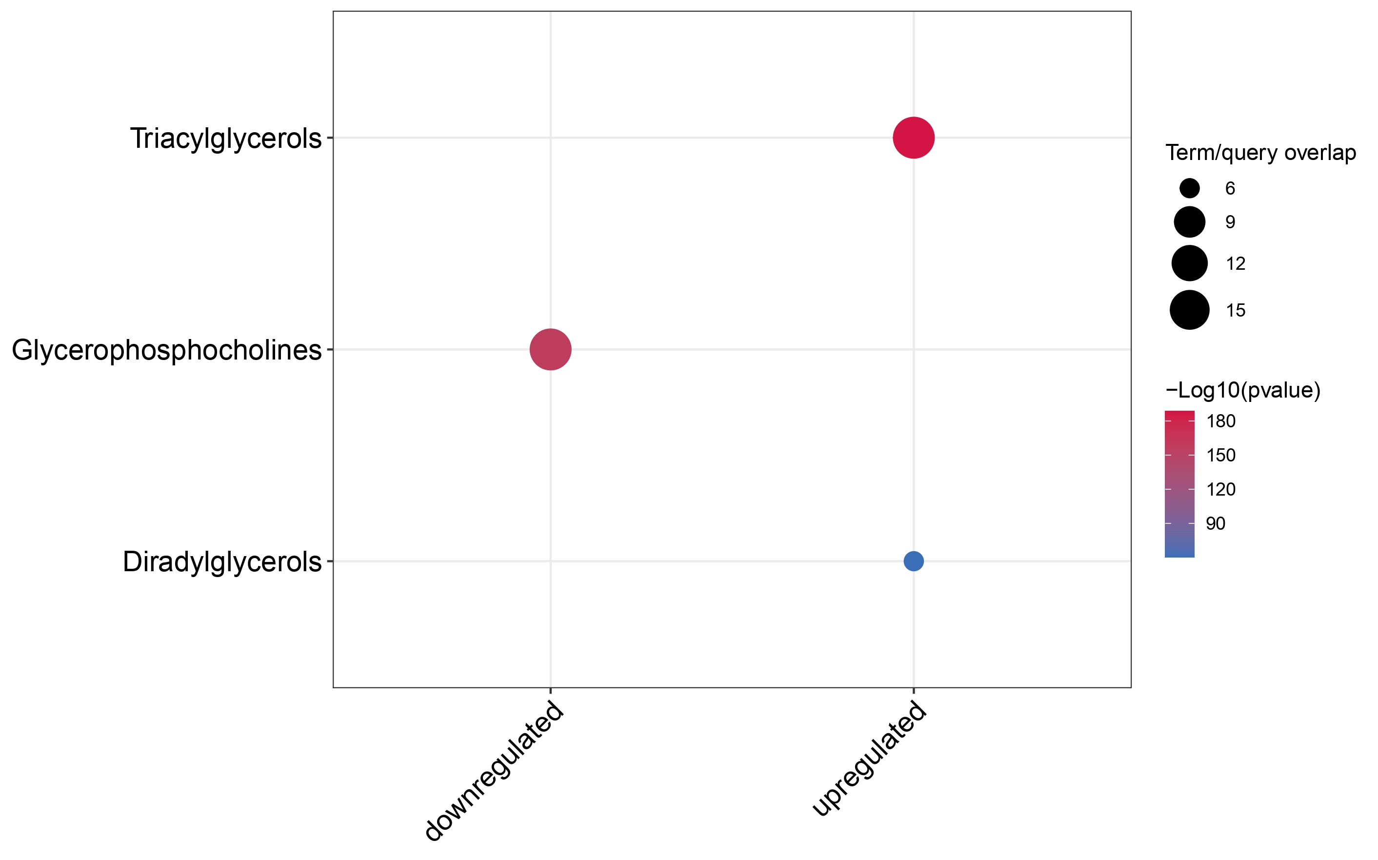

Ridge plots

To compare the distribution of term/query overlap size across bootstraps we can plot the distribution of the overlap size across terms of interest. Here we use ridge_bootstraps function to plot the distribution of the terms enriched in both upregulated and downregulated markers found in multi_cond_collapse using the upregulated results only.

ridge_bootstraps(enrich_res = multi_cond_collapse$unfiltered_enrich_res,
                 terms_of_interest = c(multi_cond_collapse$clean_enrich_res$Term),
                 condition = "upregulated")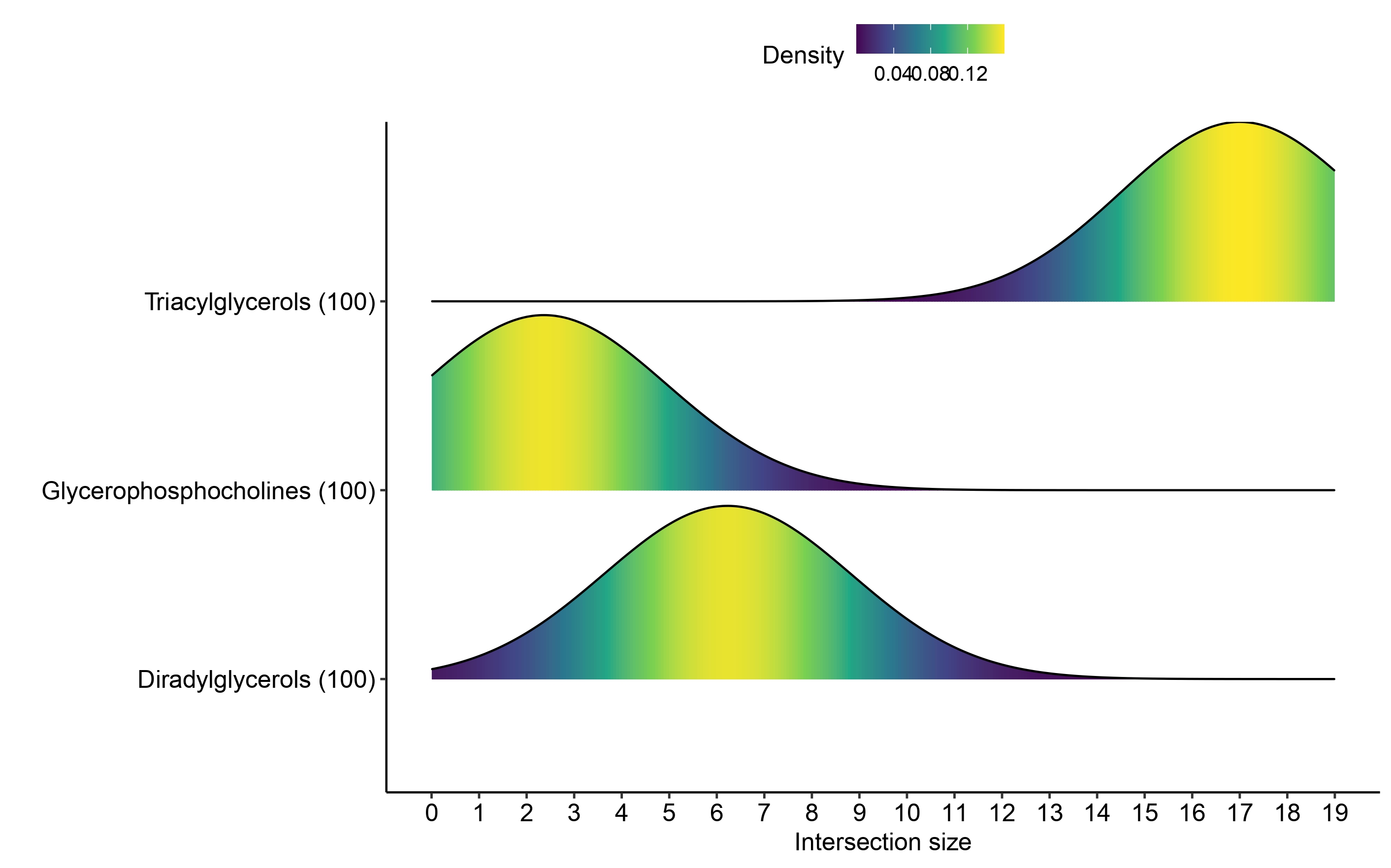

Comparative distribution of marker ions

We also provide a simple function to get the TP markers associated with a given term which correspond to the input ion in the input_scm matrix used as input.

TP_ions = get_TP_markers_per_Term(ORA_boot_df = ORA_boot_res$downregulated$unfiltered_enrich_res,
                                  term_of_interest = "Glycerophosphocholines")
TP_ions = map_TP_markers_to_ions(markers = TP_ions,
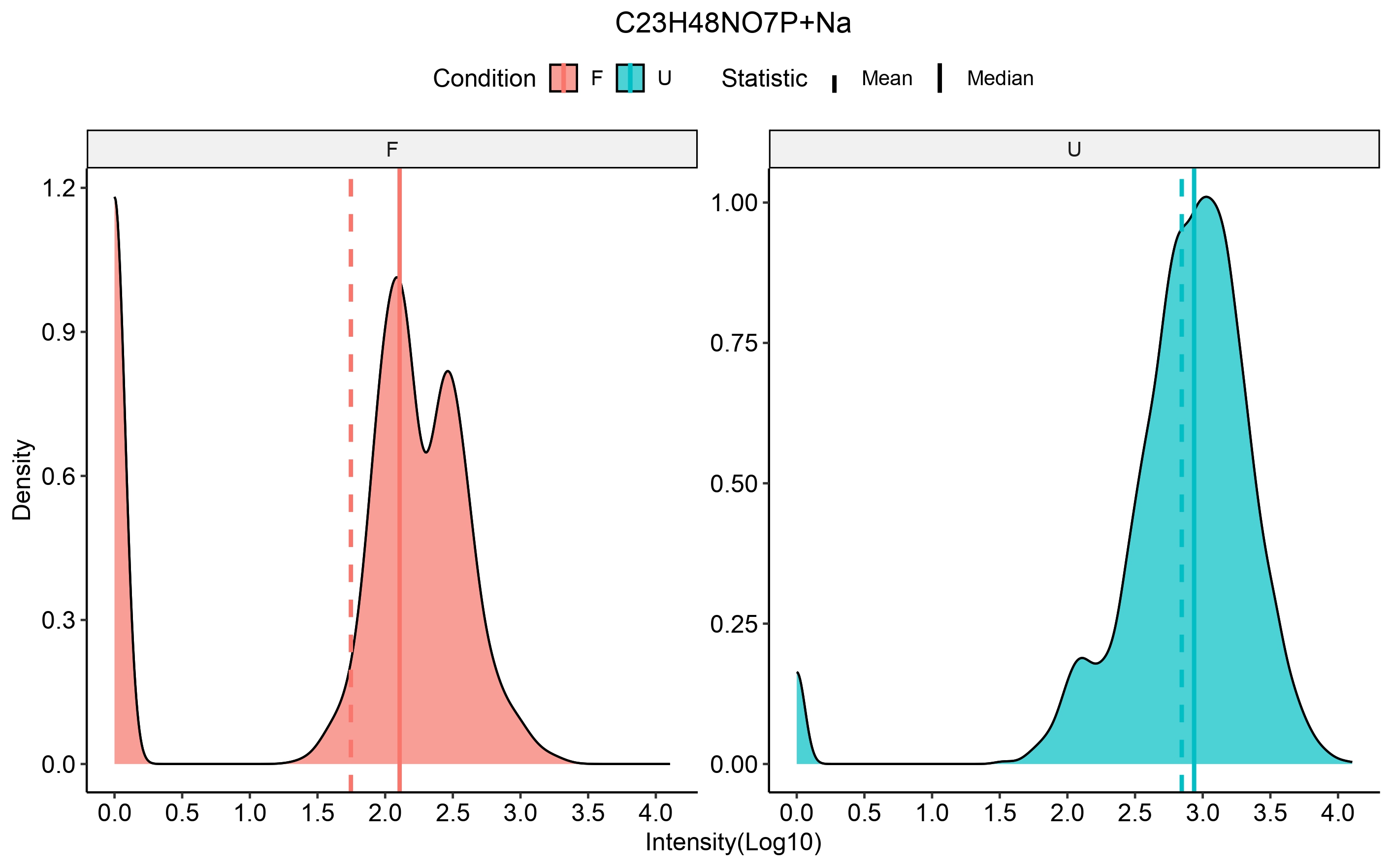
                                 scm_ions = rownames(input_scm))

We can then select an ion of interest to check distribution of intensities in the specified conditions using the compare_metabo_distr function which takes the ORA_boot_obj as input, the ions and the conditions of interest.

compare_metabo_distr(ORA_boot_obj, metabolite = TP_ions[5],
                     conds_of_interest = c(cond_x, cond_y))

ORA enrichment - single cell metabolomics

Bishoy Wadie